There’s more than one way to skin a cat

In a previous post we examined at the strange looking log function that we are supposed to minimise to win the $3 million HHP and showed that all errors are not equal with this metric.

For example, a difference of 0.1 between your prediction and the actual value is more severely punished if the actual is 0 than if the actual is 15. The point of this is because it is more important to know if the customer is going to go to hospital or not than knowing exactly how many days they will be in hospital.

Now this 'non-standard' way the model is being judged might cause issues if we are using standard algorithms that seek to minimise different error functions. For example, in linear regression, the algorithm seeks to find a solution that minimises the sum of the squared errors, with no regard for what the actual value is;

sqrt( ( pred - act ) ^ 2 )

So, does this mean that we have to come up with a new algorithm that seeks to minimise this specific log function, or is there anything else that can be done so that we don't have to reinvent the wheel? 

Now the error function we are asked to minimise is very similar,

sqrt(  (  log(pred+1) - log(act+1)  ) ^ 2  )

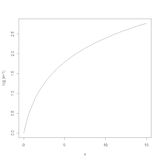
Note that the fact we have taken the log(act+1) is what introduces the issue that the magnitude of the actual value plays a part. The plot below shows x v log(x+1). A small change in x will give different changes in log(x+1) depending on what x was in the first place (ie the gradient of the line).

So, what to do?

If we look at the two equations above we can see that they are the same if we substitute

pred1 = log(pred + 1) and act1 = log(act + 1)

So, if rather than predict DIH, we predict log(DIH + 1), then we can use least squares minimisation, and use some standard algorithms that have already been developed for us. 

What we need to remember though is that when we make a submission we have put the prediction back on the right scale.

DIH_tran = log(DIH + 1)

DIH + 1 = exp(DIH_tran)

DIH = exp(DIH_tran) - 1

If we plot the data with these adjustments we can see how the error surface shows parallel lines, meaning all errors are equal, and least squares minimisation will work OK. When we put the errors back on the original scale, all errors are not equal. 

#############################################
# NOW ADJUSTING THE TARGET SO WE CAN
# MINIMISE THE RMSE
#############################################


# generate the data
dih <- seq(from=0, to=15, by = 0.05)

#adjusted days in hospital
dih1 <- log(dih + 1)
dat <- expand.grid(act1 = dih1, pred1 = dih1)

#adjusted error function
dat$err1 <- sqrt((dat$pred1 - dat$act1) ^ 2)

#'un-adjust' the days in hospital
dat$act <- exp(dat$act1) - 1 
dat$pred <- exp(dat$pred1) - 1

#plot the error on the adjusted scale
contourplot(err1 ~ act1 * pred1, data = dat
          ,region = TRUE
          ,cuts = 10
          ,col.regions = terrain.colors
          )
    
#plot the real scale
contourplot(err1 ~ act * pred, data = dat
          ,region = TRUE
          ,cuts = 10
          ,col.regions = terrain.colors
          )