Another New Comp
Kaggle have just posted a new competition Dunnhumby's Shopper Challenge that is a very interesting one. The data is historical records of when customers visited a store and how much they spent. The goal is to predict when customers will next visit the store and how much they will spend.
This is probably a novel real world data set and I expect the interest in this competition to be high. The reasons I think this are
So, where to start?
The first thing I always do is run the data through my Nifty Tool (see here for example) to check it and generate some SQL so I can load it into a database.
Here is what comes out...
Now Lets Look at the Data
In order to get a feel for things, we will aggregate the data to a daily level and look at how the population as a whole goes shopping. We will create a count of the total number of visits per day and generate some time based fields that will help us understand the daily and seasonal patterns in shopping. The SQL below will generate that data, which is small enough to save in Excel or as a text file and then load in your favourite analysis package, or we could just create a table in the database and load directly from there (don't leave as a view as it takes a while to generate).
Tiberius is an ideal tool for analysing this type of data, as I initially wrote it to look at a similar type of data set - electricity consumption - and the patterns I want to discover will be similar.
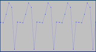
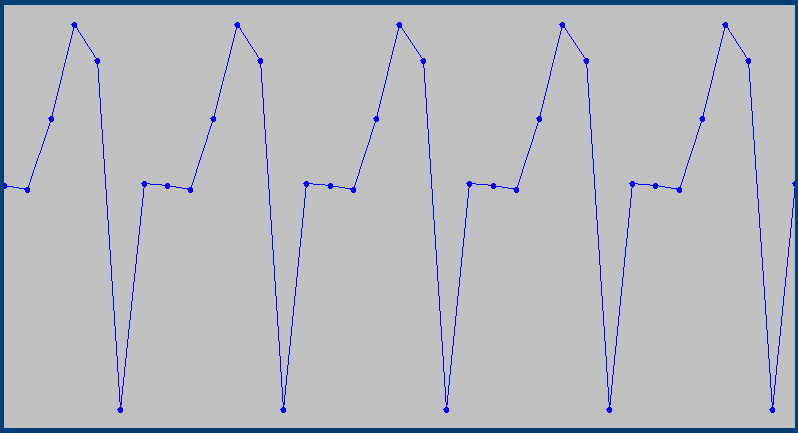
I have built a model to predict visits as a function of time. The model predictors are weekly, seasonal and trend components, so we are trying to model the number of visits based solely on time. The plot below shows the errors in the model, the points are in date order.
(Click on the plots to enlarge)

What we see are that there are certain dates where the errors stand out. These are easily identifed in Tiberius by rolling your mouse over the image and the dates are displayed.
The two big anomalies are 25th Dec 2010 and 1st Jan 2011 - Christmas Day and New Years Day. So if we are trying to deduce where this data set is from, China is probably crossed off the list.
Other dates with errors are
A bit of research will identify that these are all England & Wales public holidays, so I think we have figured out where the data set originates from (hello Tesco!).
The model of visits can be decomposed into weekly, annual and a trend components.
The weekly component shows Sunday is the quietest day, and Friday the busiest day. Monday, Tuesday and Wednesday are all similar.
The Seasonal component shows early April is the busiest time of year.

And unfortunately the trend looks to be going downhill.

Finally here is an interesting plot of the standard deviation of the spend,

So we are on our way to understanding this problem.
Good luck everyone, hope the challenge keeps you busy!
Kaggle have just posted a new competition Dunnhumby's Shopper Challenge that is a very interesting one. The data is historical records of when customers visited a store and how much they spent. The goal is to predict when customers will next visit the store and how much they will spend.
This is probably a novel real world data set and I expect the interest in this competition to be high. The reasons I think this are
- The data is simple
- There is not a massive amount of data, so processing power will not be an issue
- It is a novel problem where creativity is needed and a new algorithm will probably have to be developed. It is not going to be a case of who can pre-process the data best and build the best ensemble using existing algorithms
So, where to start?
The first thing I always do is run the data through my Nifty Tool (see here for example) to check it and generate some SQL so I can load it into a database.
Here is what comes out...
CREATE DATABASE dunnhumby
USE dunnhumby

CREATE TABLE training
(
    customer_id    int
,    visit_date    date
,    visit_spend    float
)


BULK INSERT training
FROM 'E:\comps\dunnhumby\training.csv'
WITH
(
MAXERRORS = 0,
FIRSTROW = 2,
FIELDTERMINATOR = ',',
ROWTERMINATOR = '\n'
)

--(12146637 row(s) affected)


CREATE TABLE test
(
    customer_id    int
,    visit_date    date
,    visit_spend    float
)


BULK INSERT test
FROM 'E:\comps\dunnhumby\test.csv'
WITH
(
MAXERRORS = 0,
FIRSTROW = 2,
FIELDTERMINATOR = ',',
ROWTERMINATOR = '\n'
)
The data set is relatively nice, just 3 coulumns;
- customer ID
- date
- amount spent
the dates are from 1st April 2010 to 18th July 2011.
A Naive Guess
I always like to get in a submission without actually really looking at the data, just to make sure I am reading the data correctly and that the submission file is in the correct format.
In forecasting, a naive prediction is not going to be far wrong in the long run. If you want to forecast the weather, then saying tomorrow is going to be the same as today is going to serve you well in the long run if you have no other information to go off. So for this problem, we will say the next spend will be the same as the last spend, and the gap in days will also be the same.
To achieve this in SQL is a bit tricky, but can be done. The code below does the trick and when submitted gets 9.5% correct on the leaderboard, the same as the simple baseline benchmark.
/*************************************************
SQL to generate a naive prediction
- spend will be the same as the last visit
- the next visit will be in the same number
  of days as the gap between the previous visit
**************************************************/

-- append a visit number to the data - visit 1 = most recent visit
select *, Rank() over (Partition BY customer_id order by visit_date desc) as visit_number
into #temp1
from test

-- create field which is days since previous visit
select a.*
,b.visit_date as previous_visit_date
,DATEDIFF(DD,b.visit_date,a.visit_date) as days_since_previous_visit
into #temp2
from #temp1 a inner join #temp1 b
on a.customer_id = b.customer_id
and a.visit_number = b.visit_number - 1
where a.visit_number = 1

-- generate the submission file, makink sure 1st April is earliest data
select
customer_id
,
    (case
        when dateadd(dd,days_since_previous_visit,visit_date) < '2011-04-01'
        then '2011-04-01'
        else dateadd(dd,days_since_previous_visit,visit_date)
    end)
    as visit_date
,visit_spend
from #temp2
order by customer_id
Now Lets Look at the Data
In order to get a feel for things, we will aggregate the data to a daily level and look at how the population as a whole goes shopping. We will create a count of the total number of visits per day and generate some time based fields that will help us understand the daily and seasonal patterns in shopping. The SQL below will generate that data, which is small enough to save in Excel or as a text file and then load in your favourite analysis package, or we could just create a table in the database and load directly from there (don't leave as a view as it takes a while to generate).
-- add a field which is the days since 1st April (1st April 2010)
alter table training add daysSinceStart int
update training set daysSinceStart = DATEDIFF(dd,'2010-04-01',visit_date)

-- create a daily summary dataset
select visit_date

-- fields of interest
, COUNT(*) as visits
, avg(visit_spend) as avg_visit_spend
, stdev(visit_spend) as stdv_visit_spend

-- time based predictor variables
, min(daysSinceStart) as daysSinceStart
, sin(2 * pi() * (DATEPART(DAYOFYEAR, visit_date) * 1.0 / 365.0)) as doySin
, cos(2 * pi() * (DATEPART(DAYOFYEAR, visit_date) * 1.0 / 365.0)) as doyCos
, (case when (DATEPART(WEEKDAY, visit_date)) = 1 then 1 else 0 end) as dowSun
, (case when (DATEPART(WEEKDAY, visit_date)) = 2 then 1 else 0 end) as dowMon
, (case when (DATEPART(WEEKDAY, visit_date)) = 3 then 1 else 0 end) as dowTue
, (case when (DATEPART(WEEKDAY, visit_date)) = 4 then 1 else 0 end) as dowWed
, (case when (DATEPART(WEEKDAY, visit_date)) = 5 then 1 else 0 end) as dowThu
, (case when (DATEPART(WEEKDAY, visit_date)) = 6 then 1 else 0 end) as dowFri
, (case when (DATEPART(WEEKDAY, visit_date)) = 7 then 1 else 0 end) as dowSat

from dbo.training
group by visit_date
order by visit_date asc
Tiberius is an ideal tool for analysing this type of data, as I initially wrote it to look at a similar type of data set - electricity consumption - and the patterns I want to discover will be similar.
I have built a model to predict visits as a function of time. The model predictors are weekly, seasonal and trend components, so we are trying to model the number of visits based solely on time. The plot below shows the errors in the model, the points are in date order.
(Click on the plots to enlarge)

What we see are that there are certain dates where the errors stand out. These are easily identifed in Tiberius by rolling your mouse over the image and the dates are displayed.
The two big anomalies are 25th Dec 2010 and 1st Jan 2011 - Christmas Day and New Years Day. So if we are trying to deduce where this data set is from, China is probably crossed off the list.
Other dates with errors are
- 4th April 2010
- 3rd May 2010
- 31st May 2010
- 30th August 2010
A bit of research will identify that these are all England & Wales public holidays, so I think we have figured out where the data set originates from (hello Tesco!).
The model of visits can be decomposed into weekly, annual and a trend components.
The weekly component shows Sunday is the quietest day, and Friday the busiest day. Monday, Tuesday and Wednesday are all similar.
The Seasonal component shows early April is the busiest time of year.

And unfortunately the trend looks to be going downhill.

Finally here is an interesting plot of the standard deviation of the spend,

So we are on our way to understanding this problem.
Good luck everyone, hope the challenge keeps you busy!
Hi Phil
ReplyDeleteDid you build those timeseries components in SQL or is this a feature of Tiberius?
Shane
The day flags and cycling annual term were done in SQL - see the 3rd code window above.
ReplyDeletecan you provide the data sets??
ReplyDeleteyou can get them from Kaggle
ReplyDeletehttp://www.kaggle.com/c/dunnhumbychallenge
The datasets have been removed. Can you provide them?
ReplyDeletenope - you will have to contact Kaggle
Delete