So far with the HHP I have
Data lives in a database, but it is no good to anyone if we can't get at it to analyse. It is possible to access this data, as the database developers have very genourosly provided what are called database drivers that allow these other applications to get to the data, and even change it if so desired. Many analytic applications have provided the means to utilise these drivers so the data can be sucked into their tools for analysis.
The task of connecting your applications to databases can be very painful if you are not really a database person and don't understand the lingo of what you are being asked to do. Some applications make it very easy (I have found Tableau remarkably painless and my own software Tiberius has instructions on how to do this) and some you have to Google around a lot find the answers to your questions. It is amazing how many products in their documentation just say 'contact your system administrator' - which is no help if it is you.
In the end though, once you have connected that is the biggest hurdle over, and then the world is your oyster.
So, we now want to connect SQL Server to R. First the code, then the detail.
Note: If you are viewing this in Internet Explorer or Chrome, you might get text wrapping in the code below and no horizontal scroll bar. If you are using FireFox then you get the scroll bar and no text wrapping. Either way you can still copy and paste the code OK. Another Damn Computer!
The code above is R code and is run from R. It assumes you have the library RODBC installed. If you don't, then just type
There are 2 options to connect to the database, methods 1 & 2.
In method 1, you need to know 3 bits of information (you also might need user IDs and passwords depending on how access to the database is set up),

The end result of all this is that we can connect R to our database and plot a graph. We can now get a sense of what the data is all about. Progress!
Interesting observations - Days in Hospital is mainly 0, then 1-5, with another hardly visible blip at 15.


Interesting, obviously an anomaly in the data? Or maybe we should now start to read about the problem we are trying to solve and how the data has been put together.
We can just change the query to look at a different table in the database. The Claims data looks like this...

This gives us an idea of what we are dealing with. Now to 'shake rattle and roll!'
- loaded the data into a database
- written an R script to check the submission file is correct, with the added bonus of plotting a distribution for a sanity check
Data lives in a database, but it is no good to anyone if we can't get at it to analyse. It is possible to access this data, as the database developers have very genourosly provided what are called database drivers that allow these other applications to get to the data, and even change it if so desired. Many analytic applications have provided the means to utilise these drivers so the data can be sucked into their tools for analysis.
The task of connecting your applications to databases can be very painful if you are not really a database person and don't understand the lingo of what you are being asked to do. Some applications make it very easy (I have found Tableau remarkably painless and my own software Tiberius has instructions on how to do this) and some you have to Google around a lot find the answers to your questions. It is amazing how many products in their documentation just say 'contact your system administrator' - which is no help if it is you.
In the end though, once you have connected that is the biggest hurdle over, and then the world is your oyster.
So, we now want to connect SQL Server to R. First the code, then the detail.
Note: If you are viewing this in Internet Explorer or Chrome, you might get text wrapping in the code below and no horizontal scroll bar. If you are using FireFox then you get the scroll bar and no text wrapping. Either way you can still copy and paste the code OK. Another Damn Computer!
# load the required libraries
library(RODBC) #for data connection
library(lattice) #for histograms

#######################################
# set up a connection to the database
#######################################

#method 1 - using a connection string
conn <- odbcDriverConnect("driver=SQL Server;database=HHP;server=PHIL-PC\\SQLEXPRESS;")

#method 2 - involves setting up a DSN (Data Source Name)
#conn <- odbcConnect("sql_server_HHP")


########################################################
# extract the data using this connection and some SQL
########################################################
mydata <- sqlQuery(conn,"select  * from DaysInHospital_Y2")
#mydata <- sqlQuery(conn,"select  * from Claims")


############################
# take a look at the data
############################
colnames(mydata)
head(mydata)
summary(mydata)


############################
# plot the distributions
############################

#set up the plot layout
maxplots <- 9 #upper limit on plots
plots <- NCOL(mydata)
plots <- min(plots,maxplots)
sideA <- ceiling(sqrt(plots))
sideB <- ceiling(plots/sideA)
cells <- sideA * sideB
#par(mfrow=c(sideA,sideB)) #use this for standard graphics
plotposition <- matrix(1:cells,sideA,sideB,byrow = T)

#draw all the plots
for(i in 1:plots){
myplot <- histogram(mydata[,i],main=colnames(mydata[i]),xlab='')
myposition <- rev(which(plotposition == i, arr.ind=TRUE))
print(myplot, split=c(myposition,sideA,sideB), more=TRUE)
}
The code above is R code and is run from R. It assumes you have the library RODBC installed. If you don't, then just type
install.packages('RODBC')
So, how do you get it to work?
There are 2 options to connect to the database, methods 1 & 2.
In method 1, you need to know 3 bits of information (you also might need user IDs and passwords depending on how access to the database is set up),
- the driver name (SQL Server in our case)
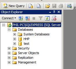
- the database server name. This can be tricky to remember. For SQL Server the easiest way to find it is when you start up the SQL Server Management Studio. In the picture below you will see the server name is PHIL-PC\SQLEXPRESS.

There is one gotcha here. You will notice in the R script we have an extra '\'
server=PHIL-PC\\SQLEXPRESS
This is because '\' is a special charater in R, so you need to put two of them together to tell it that you really do mean '\'. This is useful to know when you have paths of files etc.
Another thing to note above, we are in Windows Authentication mode, which means we won't have to worry with passwords. - The name of the database in the database server that you want to connect to. You can discover your options from within the Management Studio. Here we have HHP and test

So when we string all this together we get,
conn <- odbcDriverConnect("driver=SQL Server;database=HHP;server=PHIL-PC\\SQLEXPRESS;")
Method 2 involves creating a Data Source Name (DSN), which can be thought of as the above bits of information but stored away somewhere in your computer, just wrapped under a name. With many applications, you just then have to specify this name to connect to the data.
On Windows machines, a DSN is created via a wizard that takes you through the steps. Here are instructions for XP.
The one Gotcha that I commonly encounter with SQL Server is that it tries to populate the list of available servers so you can just select it from a list, sometimes you can be waiting forever and you are not guaranteed to get your server in the list.

You can see above that it lists PHIL-PC, but this will fail, it needs to be PHIL-PC\SQLEXPRESS.
Also, if you are connected to a network, the list of servers could be pretty big and picking the one you need would be difficult to remember. If you do this often it can be worthwhile just having your common servers in a list and just pasting them in.
With the wizard, it can test the connection for you, so you know if your settings are correct.
The end result of all this is that we can connect R to our database and plot a graph. We can now get a sense of what the data is all about. Progress!
Interesting observations - Days in Hospital is mainly 0, then 1-5, with another hardly visible blip at 15.


hist(mydata$DaysInHospital[mydata$DaysInHospital > 1])

Interesting, obviously an anomaly in the data? Or maybe we should now start to read about the problem we are trying to solve and how the data has been put together.
We can just change the query to look at a different table in the database. The Claims data looks like this...

This gives us an idea of what we are dealing with. Now to 'shake rattle and roll!'
Awesome post. why not just use par(mfrow=c(3,3)) though?
ReplyDeleteHi Tanya,
ReplyDeleteThat was my initial attempt, but it did not work. Apparently the lattice package does not respect par settings.
If you try it you will see what happens.
Hi Phil
ReplyDeleteI am following your posts. How is one supposed to handle the values '15+' : by converting to '15' or '16' ? As otherwise R interprets this column as a category. Also, this conversion needs to be done outside R - there doesnt seem to be a conversion facility while reading data??
I do all my data manipulation outside of R, basically because there are other tools I am more familiar with, but it would be simple to do it all in R.
ReplyDeleteIf you convert 15+ to 15 or 16 doesn't really matter - depending on what modelling algorithm you are using. Tree based methods won't make a difference, linear regression type models it might.
The code below is an example of how I did some conversion in SQL.
----------------------
-- charlesonindex
----------------------
--select distinct CharlsonIndex from claims
alter table claims
add CharlsonIndexI INTEGER
go
update claims
SET CharlsonIndexI =
CASE
when CharlsonIndex = '3-4' then 4
when CharlsonIndex = '5+' then 6
when CharlsonIndex = '1-2' then 2
when CharlsonIndex = '0' then 0
end